TrainingSkills

This blog is an intro about several practical approach for training models.

Data preprocessing#

Why do we need preprocess#

• Activation functions (ReLU) works around zero

If input data is biased toward positive or negative, randomly initialized layers produce biased output.

• A feature with small scale has a negligible effect on backprop.
• Remove correlation between input features (PCA Whitening)

And a lot more …

Normalizations#

Normalization : Normalize the distribution of activations to have zero mean and unit variance

Why we shall do normalization:

• Internal Covariate Shift

provides the theoretical basis for why normalization is necessary—it stabilizes the input distribution to layers and speeds up learning.

• To Train Deeper Networks on Larger Data

For deeper networks and larger datasets, normalization improves training stability, enhances convergence speed, and ensures better performance.

Batch Normalization#

[Ioffe and Szegedy, 2015]

Why it is good?

• Improves gradient flow
• Allows higher learning rates
• Reduces strong dependence on initialization
• Regularization

Usually added after convolutional layers or fully connected layers && before non-linearities

Missing Datapoint#

Missing data can be handled in several ways:

1. Imputation: Replace missing values with a statistic like mean, median, or
   mode, or use a model to predict missing values.
2. Removal: If the missing values are not random or comprise a large portion
   of the data, it might be better to remove those points.
3. Indicator Variable: For some algorithms, it can be useful to create a new
   variable indicating the presence of missing data along with imputation.

Activation Functions#

Conclusion First:

• Use ReLU. Be careful with your learning rates

• Try out Leaky ReLU / Maxout / ELU

  To squeeze out some marginal gains

• Don’t use sigmoid or tanh

Don’t use sigmoid or tanh#

• Sigmoid:

  • Formula: $\sigma(x)=\frac{1}{1+e^{-x}}$
  • Outputs values between 0 and 1.
  • Problems:
    • Vanishing gradients: For large positive or negative inputs, the gradient becomes very small, slowing down learning.
    • Outputs are not zero-centered: This can cause inefficient gradient updates.

• Tanh:

  • Formula: $\tanh(x)=\frac{\sinh(x)}{\cosh(x)}=\frac{e^x-e^{-x}}{e^x+e^{-x}}$
  • Outputs values between -1 and 1.
  • Problems:
    • Vanishing gradients: Like sigmoid, tanh saturates for large positive or negative inputs.
    • Slightly better than sigmoid because it’s zero-centered, but still inferior to ReLU and its variants.

• Why avoid them:

  • Modern networks prefer ReLU or its variants because they avoid these issues, train faster, and perform better for deep architectures.

Use ReLU. Be careful with your learning rates#

• ReLU (Rectified Linear Unit):

  • ReLU is one of the most commonly used activation functions in deep learning because it introduces non-linearity while being computationally efficient.
  • Defined as: $\mathrm{ReLU}(x)=\max(0,x)$, it outputs the input directly if positive and zero otherwise.

• Why ReLU is recommended:

  • Sparse activation: Only a subset of neurons are activated at any given time, making the network more efficient.
  • Avoids vanishing gradients: Unlike sigmoid or tanh, ReLU doesn’t squash gradients, which helps deeper networks learn effectively.

• Caution about learning rates:

  • Problem: ReLU can cause the “dead neuron” problem, where some neurons output zero for all inputs and stop learning. This happens when the input to the ReLU is consistently negative due to high learning rates.
  • Solution: Use a moderate learning rate and techniques like proper weight initialization or adaptive optimizers (e.g., Adam).

Experiment with Leaky ReLU, Maxout, or ELU for improved performance or to avoid specific issues with ReLU.#

Focus on incremental improvements when the model is already performing well.

• Leaky ReLU:

  • A variant of ReLU that allows a small, non-zero gradient for negative inputs, preventing the “dead neuron” problem.
  • Formula: $\text{Leaky ReLU}(x)=\left\{\begin{array}{lll}x & x>0\;\alpha x & x\le 0\end{array}\right.$, where $\alpha$ is a small positive constant (e.g., 0.01).

• Maxout:

  • Generalizes ReLU and allows learning the activation function directly.
  • Formula: $\mathrm{Maxout}(x)=\max(w_T^1x+b_1,\,w_T^2x+b_2)$, where $w_1,\,w_2$ are learnable parameters.
  • Benefits: Provides greater flexibility in modeling but increases the number of parameters.

• ELU (Exponential Linear Unit):

  • Smooths out the ReLU function for negative values, providing better gradient flow.
  • Formula: $\mathrm{ELU}(x)=\left\{\begin{array}{lll}x & x>0\;\alpha(\exp(x)-1) & x\le 0\end{array}\right.$, where $\alpha>0$ controls the curve for negative values.
  • Negative saturation regime compared with Leaky ReLU adds some robustness to noise

Weight Initialization#

$Y=W*x$
If all weights in W are 0 , Output Ywill be always 0 and then gradients will go to 0, causing gradient vanishing problem.

There are several existing approach to deal with initialization:

Small Random Numbers(Doesn’t work for deeper networks)#

Sample from a gaussian distribution with 0 mean and given standard deviation (such as 0.01)

$W\sim N(\mu,\sigma^2)$

W = 0.01*np.random.randn(Din,Dout)(for conv layers, Din is ${fiter_s ize}^{2}*input_c hannels$)

Why not working for deeper networks?

After several forward pass, the X will be 0 mean and negligible std.

W = 0.01*np.random.randn(Din,Dout)
x = tanh(x@W)

==> after 6 forward pass
x = x@W@W@W@W@W@W

Xavier Initialization#

Approach: Set the variance according to # of input neurons

Intuition: input and output with the same variance to prevent vanishing or exploding problem

$W\sim N(\mu,\sigma^2)$ and $Var(W)=\frac{1}{D_{in}}$

W = np.random.randn(Din,Dout)/np.sqrt(Din)

Let: $y=x_1w_1+x_2w_2+\cdots+x_{D_{in}}w_{D_{in}}$

Assume:

We want:

So,$Var(y)=Var(x_i)$ only when $Var(W)=\frac{1}{D_{in}}$

While for ReLU, activations collapse to zero again, no learning.

Kaiming Initialization#

For a layer with input dimension $D_{in}$ (number of input neurons), the weights are initialized as:

This means:

• The weights are drawn from a normal distribution with a mean of 0 and a variance of $\frac{2}{D_{in}}$.
• The scaling factor $\frac{2}{D_{in}}$ accounts for the ReLU activation function, ensuring that the variance of the outputs remains stable as it propagates through the network.

Kaiming initialization is particularly effective when using ReLU, Leaky ReLU, or similar activation functions that introduce sparsity. For networks with sigmoid or tanh activations, Xavier initialization is typically preferred.

Optimization#

Momentum + SGD#

SGD:

loop:
    dx = compute_gradient(x)
    x -= learning_rate * dx

SGD + Momentum:

vx = 0
loop:
    dx = compute_gradient(x)
    vx = rho*vx + dx
    x -= learning_rate * dx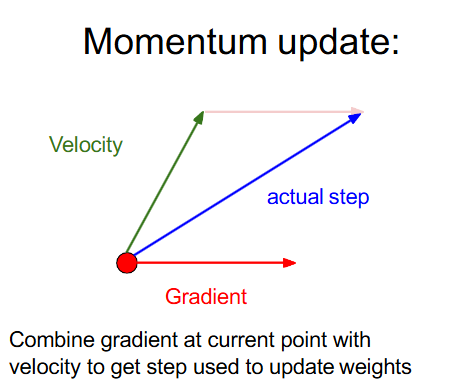

Reduce the oscillations in the rapid change directions. (Avoid zig-zag)

AdaGrad#

grad_squared = 0
loop:
    dx = compute_gradient(x)
    grad_squared += dx * dx
    x -= learning_rate * dx / (np.sqrt(grad_squared) + 1e-7)

Such that:

1. Progress along “steep” directions is damped
   progress along “flat” directions is accelerated
2. After long time, $\Delta(x)\to 0$

RMSProp:

grad_squared = 0
loop:
    dx = compute_gradient(x)
    grad_squared = decay_rate * grad_squared + (1 - decay_rate) * dx * dx
    x -= learning_rate * dx / (np.sqrt(grad_squared) + 1e-7)

can make momentum smoother

Adams#

from RMSProp:

(Almost)

first_moment = 0
second_moment = 0
loop:
    dx = compute_gradient(x)
    first_moment = beta1 * first_moment + (1 - beta1) * dx [momentum]
    second_moment = beta2 * second_moment + (1 - beta2) * dx * dx [adagrad/RMSProp]
    x -= learning_rate * first_moment / (np.sqrt(second_moment) + 1e-7)

(Full form)

first_moment = 0
second_moment = 0
for t in range(1, num_iterations):
    dx = compute_gradient(x)

    first_moment = beta1 * first_moment + (1 - beta1) * dx
    second_moment = beta2 * second_moment + (1 - beta2) * dx * dx

    first_unbias = first_moment / (1 - beta1 ** t)
    second_unbias = second_moment / (1 - beta2 ** t)

    x -= learning_rate * first_unbias / (np.sqrt(second_unbias) + 1e-7)